> restart;

> with(plots);

> with(plottools);
readlib(isolate):

Depth of field, frame size and focus stacks
Results based on the thin lens geometric optic model

Richard Lemieux, 2021

I provide here the derivation of some useful optical formulas related to Photography. The subject is quite old. However the mirrorless digital cameras come with the challenge of estimating the DOF of a picture without the distance information and just from what the photographer sees on the LCD display or on the viewfinder and what he knows of the camera. I propose here to use the frame size as an alternative to the distance with the assumption that photographers will use approximations of the DOF numbers based on estimates of the frame size.

The original part of this note introduces a few distance-free formulas and approximations for the depth-of-field (DOF) that depend on the frame size. What do I mean by the frame size? I will also use the word canvas to denote the same concept. Imagine there is a large rectangular frame located at the position of the subject and facing the camera and that frame is rendered by the camera as the borders of the LCD and the borders of the frame displayed in the EVF. Three frames are special: 1) the frame where the subject is located, 2) the frame at the distance where the DOF is equal to the frame size and 3) the frame located at the hyperfocal distance.

All formulas here are based on the thin lens geometrical optic model. The context is digital photography where the relevant parameters are the resolution and the size of the sensor and of the displays, the focal length and the aperture of the lens and the normal viewing distance of the displays based on the pixel size. I will also mention the case where the effective image resolution is smaller than the pixel count due to optical effects in the lens.

The second part of this note is a derivation of formulas related to focus stacks. I have used the results from this note in a Lua script that estimates the number of frames to include in a stack. That number is an input parameter to the Fuji X-T3 focus stack function. The Lua script runs in the Comet Lua interpreter on Android phones or any Lua distribution.

The note is organised as follows,

1. A reminder of he basic relations of thin lens optics and the most commonly met setups.

2. A derivation of DOF formulas free of the distance variable and based on canvas.

3. The basics of focus stacks and the derivation of formulas to estimate the number of frames needed.

The idea is to provide tools that the photographer finds intuitive. The DOF formulas given here can be evaluated mentally and without the need of a calculator. The formulas can also be used in some focus stack scenarios to estimate the number of frames. At the other end of the scale an Android phone is needed to run the Lua scripts.

The computations reflect a simple model of a lens where the lens is a single thin piece of glass. Focusing is done by moving the sensor. Distances are measured positive starting from the lens position in both the right and the left directions so all-distance numbers are positive.

Abreviations used in this note.

This section provides a short description of the symbols used in the derivation of the fprmulas. Please refer to outside sources such as Wikipedia for in depth descriptions of the associated concepts.

A: Aperture diameter of the thin lens.
Av: Aperture number of the lens (2, 2.8, 4 etc. Av = A/f).

coc : Circle of confusion. Kingslake's "Lenses in Photography" has a good chapter describing the classic view on the subject. The minimal value of the coc on digital is the pixel size on the sensor. However it may be better to use the largest number between the pixel size, the resolution of the lens at the current aperture and the actual resolution of the viewing device given the expected viewing distance. Those are all easy considerations to integrate in the framework introduced in this note just by choosing the appropriate resolution number in the formulas.

D: Distance from the lens to the subject (the focus point).

Ds: Distance from the sensor to the subject.

DOF: Depth of field. The portion of the scene in the front and in the back of the subject at the focus point that looks sharp. This is a slice of the scene of thickness DOF. The slice is centered on the subject.

f: Focal lens of the lens.
FSs: Size of the short side of the frame at the focus point.

Hyperfocal distance(H) : Obects located at distances going from half the hyperfocal distance to Infinity look all in focus when the sensor focused on a subject located at the hyperfocal distance.

IS: Size of the image of the subject on the sensor (See also 'x')..

M: Magnification (M = IS/SS = SensorS/SubjectFS).

PixelC: The number of pixels matching the SensorS dimension when one is to view the picture at 1:1. Any smaller number can be used here either to account for the loss of resolution due to diffraxtion or if viewing the whole picture (not at 1:1) to reflect the actual number of pixels of the viewing screen or the viewing setup.

rDOF: Depth of field relative to the frame size at the subject location (rDOF = DOF/SubjectFS).

sharp. This is a perception of the eye of the person viewing the picture. That depends on the acuity of the eye, the distance between the viewer and the screen, and the size of the screen. A convenient viewing setting in this digital age is to view the screen from a distance where the viewer just stops resolving the individual pixels on the screen. This is very consistent with what Rudolf Kingslake wrote in his book: "Lenses for photography". When viewing the whole picture as opposed to a 1:1 crop, then one would be better using the resolution provided by the viewing setup as a value for PixelC.

SubjectFS: The size of the sensor frame projected at the subject location (either the height or the width) assuming that he focus is on the subject. I also use the word "canvas" to give it an artistic flavour when referring to the frame as if a painter was drawing on a large life sized canvas positioned just at the subject location.

SubjectFSH: The size of the frame at the focus distance where the depth of field extends to infinity (Hyperfocal).

SubjectFS1G: The size of the frame for a ratio frame_size/depth_of_field = 1. For a lens of focal length f. This is the general case.
SubjectFS1L: The size of the frame for a ratio frame_size/depth_of_field = 1. For a long focal length. This is the value used in the rDOF formula.

SensorS: Either the height or the width of the sensor, but matching the SubjectFS number.

SS: Size of the subject.

x: (x+f) is the distance from the lens to the image of the subject (see also IS and SS).

xC: (xC + f) is the distance from the lens to the image of an object when that object is located at the close end of the DOF range.

xF: Similar as xC but at the far end of the DOF range.

xH: (xH + f) is the distance from the lens to the image of the subject when the subject is at the hyperfocal distance.

Figures

Main results

The main result is a formula giving the relative depth of field as a function of the sizes of three frames: 1) The frame at the focus point (SubjectFS), 2) the frame where rDOF is 1 in the midrange between macro and hyperfocal (SubjectFS1L), and 3) the frame where rDOF becomes infinite (the hyperfocal). This formula is free of any explicit reference to distances.

Practical use in the midrange between macro and hyperfocal

I typically use the simplified formula below with a pre-computed value of SubjectFS1L.

I am going to use the Fuji X-T2 as an example. The SubjectFS1L number is fixed for a camera. It does not change whatever lens is actually mounted on the camera and it is independent of any zoom action. Of course the number changes with the f-number (Av), but I am going to compute it just for one aperture: f/8. I don't need to memorize values of SubjectFS1L at all apertures because it is easy to mentally compute the number for f/4, f/2, f/16 when one has the f/8 number. So here is the f/8 number for the X-T3,

SubjectFS1L = 4000*(15.6e-3/2)/8 = 4.05;

which I round to 4 so the field formula I use in landscape mode for the vertical direction is,

So if the picture is going to be a half-body portrait and the frame is about 1m tall then the relative DOF is 25% of the vertical dimension of the frame at f/8 and that is 25cm deep. That would be 12cm at f/4 and 6cm deep at f/2.

The above simplified formula is quite easy to use. The single input is the frame size given in meters. The frame size is easy to estimate based on what one sees in the viewfinder. The focal length of the lens can be discarded as a factor as long as the frame size is half the frame size at the hyperfocal distance or less. The focal length of the lens comes in is a factor determining the value of the hyperfocal distance in the rDOF formula above. Since the frame size at the hyperfocal is not part of the simplified formula, the focal length no longer is factor in the simplified rDOF formula.

Now comes the more technical part of the note.

1. Setup

Position the subject at distance D in front of a thin lens of focal length f and aperture diameter A. The lens forms an image at distance x + f behind the lens. If the subject size is SS, then the image size is going to be IS. Please note that the thin lens is fixed in this setup and focusing is achieved by moving the sensor.

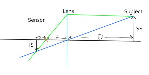
Figure1.

> eThinLensGeometry1 := SS/D = IS/(x+f);
eThinLensGeometry2 := SS/f = IS/x;
eM1 := subs(SS=IS/M, (D/IS)*eThinLensGeometry1);
eM2 := subs(SS=IS/M, (f/IS)*eThinLensGeometry2);
_1 := eliminate({eM1,eM2},M);
eD := D = solve(_1[2][1]=0,D);
dD/dx =diff(rhs(eD),x);
ex := x = solve(eD,x);
eDs := select(has,solve({ex, Ds = D+f+x})[1],Ds);
eDs2 := Ds = D*simplify(subs(eDs[1],ex,Ds/D));
eDs2D := solve(eDs2,{D});
eDs2D2 := eDs2D[1];

Relationship between the magnification (M) and the subject distance (D and Ds).

> seMfD := M = solve(subs(x=f*M,eM1),M);
seMfDs := M = solve(subs(D=Ds-(x+f),x=f*M,eM1),M);
s2eMfDs := M = 1/rhs(seMfDs)[1];
"VX33mm 1:1.4",subs(f=0.033,Ds=0.400,s2eMfDs);
"XF35mm 1:1.4";M1:=subs(f=0.035,Ds=0.280,s2eMfDs);subs(M1,FSs=(0.0156/M)*m);
"7A35mm 1:0.95";M1:=subs(f=0.035,Ds=0.370,s2eMfDs);subs(M1,FSs=(0.0156/M)*m);
"Zuiko50mm 1:1.4";M1:=subs(f=0.050,Ds=0.450,s2eMfDs);subs(M1,FSs=(0.0156/M)*m);
"#XF60mm 1:2.4";M1:=subs(f=0.060,Ds=0.267,s2eMfDs);subs(M1,FSs=(0.0156/M)*m);
"#XF18-55@18mm";M1:=subs(f=0.018,Ds=0.300,s2eMfDs);subs(M1,FSs=(0.0156/M)*m);
"#XF18-55@55mm";M1:=subs(f=0.055,Ds=0.400,s2eMfDs);subs(M1,FSs=(0.0156/M)*m);

2. Derivation of DOF formulas

2.1 Geometric relation between the depth of field (DOF) and the circle of confusion (coc)

The light coming from a small out of focus area on the scene spreads to a disk of diameter coc on the sensor. "xC" and "xF" denote the position of the focus plane for objects at the close and far ends of the in-focus zone; the object located at distance dC would be in focus if the sensor was at position xC, but the sensor is at position x and lies in front of xC (closer to the lens) and the light from the close object makes a circle of diameter "coc" on the sensor. When one chooses "coc = pixel size" the sensor does not see a difference between the objects that fall within the DOF range..

The focus distance where the depth of field is infinite is called the Hyperfocal distance. When xF = 0 in equation ecocFar, x = xH and the light coming from Infinity makes a circular patch of diameter CoC.

> eAv := Av = f/A;
ecoc := coc = SensorFS/PixelC;#The minimum size of the coc from this sensor.
ecocClose := (A/2)/(f+xC) = (coc/2)/(xC - x);#Similar triangles.
ecocFar := (A/2)/(f+xF) = (coc/2)/(x - xF);
_1 := solve(subs(A=f/Av, {ecocClose,ecocFar}),{xC,xF});
exC := select(has,_1,xC)[1];#Focus point of the close end of the DOF range.
exF := select(has,_1,xF)[1];#Focus point of the far end of the DOF range.

2.2 Depth of field (DOF), relative depth of field (rDOF) and frame size at the hyperfocal distance (SubjectFSH).

I estimate the DOF in a way that is not standard. Although not standard the method I use is based on exactly the same geometric arguments that are used to derive the standard DOF formulas. The only difference is that the standard method is based on the distance. My method (I call it mine since I didn't see it used by anyone else) is based on using a canvas (frame) at the subject location. The canvas is just the projection of the sensor at the subject position. Two canvas play a special role. First the canvas located at the distance where the DOF is equal to the canvas height. This canvas size is used to compute the relative DOF at other canvas locations. The second canvas that is special is the one located at the hyperfocal distance. The size (height) of the canvas located at the hyperfocal is the vertital resolution times the aperture diameter (focal length / f-number).
(Note) The step from eDOF3 to eDOFe is manual since my MapleV skills are still limited to the basics.

> _2 := subs(subs(D=DC,x=xC,eD), subs(D=DF,x=xF,eD), exC, exF, x=f*M, ecoc, SensorFS=SubjectFS*M, DOF = DF - DC):
eDOF := simplify(_2);
eDOF2 := simplify(subs(SubjectFS = Sf * PixelC, eDOF));
eDOF3 := subs((1+M) = M*(1/M + 1), (Sf*Av-f)*(Sf*Av+f) = -f^2*(1 - Sf^2 * Av^2/f^2), eDOF2);
eDOFe := [DOF = 2*Av*Sf*(1/M+1)/(1 - (Sf*Av/f)^2),Sf = SubjectFS/PixelC];
erDOF := subs(DOF=SubjectFS*rDOF, eDOFe[2], eDOFe[1]/SubjectFS);
erDOF2 := subs(M=SensorS/SubjectFS, erDOF);
erDOF3 := subs((SubjectFS/SensorS + 1)=(SubjectFS + SensorS2)/SensorS,erDOF2);

Derivation of SubjectFSH and SubjectFS1L from the general relative DOF formula erDOF3.

1. SujectFSH. This is the value of SubjectFS in erDOF3 when rDOF becomes infinite. That in when the factor in the denominator above is 0.

> eSubjectFSH := SubjectFSH = f*PixelC/Av;

2. SubjectFS1L. This is the value of SubjectFS in erDOF3 that makes rDOF = 1 in the region lying in between the macro range (where SubjectFS ~= SensorS) and close to the hyperfocal (when SubjectFS ~= SubjectFSH).

> eSubjectFS1L_1 := subs(rDOF=1, f=1/z, SensorS2=0, z=0, erDOF3);
eSubjectFS1L := SubjectFS1L = solve(eSubjectFS1L_1, SubjectFS);

>

At last we get 1) the general DOF formula (erDOFg) depending only on the frame sizes and 2) a simplified DOF formula (erDOFsimple) that is valid only when the focus point is not in the macro range nor close to the hyperfocal.

> erDOFg := subs(SensorS=solve(eSubjectFS1L,SensorS),f=solve(eSubjectFSH,f), SensorS2 = SensorS, erDOF3);
erDOFsimple := rDOF = SubjectFS / SubjectFS1L;

2.3 Frame size when the frame size equals the depth of field (SubjectFS1G)

I now derive an exact general formula giving the size of the frame that is equal to the DOF. That formula is good for all the values of the arguments: (f, x=SensorS/f, SubjectFS1L) -> SubjectFS1G.

> eSubjectFS1G_1 := SubjectFS1G = solve(subs(rDOF=1, SensorS2=SensorS, erDOF3), SubjectFS)[1];
eSubjectFS1G_2 := simplify(subs(PixelC=solve(eSubjectFS1L,PixelC), SensorS=x*f, eSubjectFS1G_1));
# Here I need to manually transform the results.;
eSubjectFS1G_3 := SubjectFS1G = 2*(-SubjectFS1L*Av+sqrt(SubjectFS1L*Av^2*(SubjectFS1L+SubjectFS1L*x^2-f*x^3)/(x^2))*x)/(x^2*Av);
eSubjectFS1G_4 := [SubjectFS1G = 2*SubjectFS1L*(-1+sqrt((1+x^2-SensorS*x^2/SubjectFS1L)))/(x^2), x=SensorS/f];
seq([y,subs(SensorS=0.0156, x=1/y, SubjectFS1L=4, rhs(eSubjectFS1G_4[1])/SubjectFS1L)],y=[4,2,1.5,1,0.75,.5]);
eSubjectFS1G_5 := [SubjectFS1G = 2*SubjectFS1L*(-1+sqrt((1+x^2 * (1-2*Av/PixelC))))/(x^2), x=SensorS/f];

>

3. Focus stack basic

The focus stack is a chain of frames each one focused behind the prior one. The distance between the focus points of successive frames is referred to as the StepSize. The step size such that the close end of the depth of field (DOF) range of the second frame starts exactly where the far end of the DOF range of the first frame ends is called SS1 . The points of junction where the far end of the DOF range of the close frame meets the close end of the DOF range of the next frame is called mcf below.

There are at least three focus stack scenarios depending on whether stacking is achieved by moving the sensor, the lens or both at the same time. I cover first the case where the lens is fixed and focusing is done by moving the sensor.

3.1 The lens is fixed and focusing is done by moving the sensor.

The size of the basic step size (SS1) varies with. the subject distance.

> exS2 := subs(xC=mcf,x=xS2,exC);
#Sensor position of 2nd frame (xS2) if mcf=close end of frame.
exS1 := subs(xF=mcf,x=xS1,exF);
#Sensor position of 1st frame(xS1) if mcf=far end of frame.
emcf := subs(xS2=xS1-SS1,rhs(exS1)=rhs(exS2));
# The DOF ranges of frame1(Step1) and frame2 meet here.
eSS1 := SS1 = solve(emcf,SS1); #That is the focus step.
# eSS1D := subs(SS1=SS1D,xS1=f*f/(D-f),eSS1);
# eSS1M := subs(SS1=SS1M,xS1=f*M,eSS1);

3.2 The sensor is fixed and focusing is done by moving the lens.

Each step is achieved in two movements. The first movement is to move the sensor while keeping the lens fixed as it is done above but with one difference. In the case above the focusing for the next frame is done by decreasing the x-position of the sensor until the close point of the next frame just meets the far end of the DOF range of the first frame. Here we continue moving the sensor a little garther until there is a gap G between the DOF ranges. We stop moving the sensor when the value of G is just the same as the distance traveled by the sensor. That makes us ready for the second movement.

The second movement takes the lens, the sensor and the second frame back by the length of the gap G so the sensor ends at the same position it was before the first movement.

> exS2L := subs(xC=mcf-xGap/2,x=xS2,exC);
#Sensor position for 2nd frame (xS2) if close end of frame + G/2 is the meeting point.
exS1L := subs(xF=mcf+xGap/2,x=xS1,exF);
#Sensor position of 1st frame(xS1) if mcf=far end of frame.
emcf := subs(xS2=xS1-SS1,rhs(exS1L)-xGap/2=rhs(exS2L)+xGap/2);
# The DOF ranges of frame1 (Step1) and frame2 meet here.
edDdx := dDdx = subs(x=xS1,diff(rhs(eD),x));
eSS1 := SS1 = solve(subs(xGap=SS1/dDdx,emcf),SS1); #That is the focus step.
simplify(subs(edDdx, eSS1));

Adjustment for the setup where the sensor is fixed and the lens moves.

xC: close end of DOF range.

xF: far end of DOF range.

>
exF_1L := subs(xF=mcf-dl/2,x=x_1,exF);
exC_2L := subs(xC=mcf+dl/2,x=x_2,exC);
emcfL := subs(x_2=x_1-SS1,rhs(exF_1L)+dl/2=rhs(exC_2L)-dl/2);
eSS1L := SS1 = solve(emcfL,SS1);
edl := dl = solve(subs(SS1=dl,eSS1L),dl);
simplify(subs(edl, eSS1L));
# SS1DL := dl = subs(SS1=SS1D,xf1=f*f/(D-f),eSS1L);
# eSS1ML := subs(SS1=SS1M,xf1=f*M,eSS1L);

>

> ex,exF;
eDmcf1 := solve(subs(subs(x=xF,D=Dmcf-dl/2,ex), x=x_1, exF),Dmcf);
eDmcf2 := solve(subs(subs(x=xC,D=Dmcf+dl/2,ex), x=x_1-SS1, exC),Dmcf);
eSS1L2 := SS1 = solve(eDmcf1=eDmcf2, SS1);
#edl2 := solve(subs(SS1=dl,eSS1L2),dl);
#simplify(subs(dl=edl2[1], eSS1L2));

>

> ex,exF;#Far end of the DOF range on the sensor side.
eDxF := DxF_1 = solve(subs(subs(x=xF,D=DxF_1,ex), x=x_1, exF),DxF_1);
eDxC := DxC_2 = solve(subs(subs(x=xC,D=DxC_2,ex), x=x_1-SS1, exC),DxC_2);
exC2MxF1 := xC_2MxF_1 = simplify(rhs(eDxC)-rhs(eDxF));
ed1 := dDxC/dSS1 =simplify(diff(rhs(exC2MxF1),SS1));
ed2 := d2DxC/d2SS1 =simplify(diff(rhs(ed1),SS1));
#simplify(solve(rhs(exC2MxF1)=SS1,SS1)[1]);

Focus stack with Fujifilm X-T3.
to review

> e1Steps := Steps = x/(2*Av*CoC);
eLensX := x=f^2/(D-f);
eLensXpf := map(u->f+u, eLensX);
e1D := subs(SS=CanvasHeight,IS=SensorHeight,D=solve(eThinLensGeometry1,D));
e2D := subs(eLensXpf,e1D);
e3D := D = solve(e2D,D)[2];
e2Steps := simplify(subs(eLensX,e3D,e1Steps));
e3Steps := subs(CoC=SensorHeight/PixelH, e2Steps);
e4Steps := subs(PixelH = CanvasHyperfocal*Av/f,e3Steps);
e5Steps := subs(eLensX,e1Steps);

Focus stack.
s : step size
x : position of sensor relative to focal point.
c : circle of confusion.

A ; f-number.

> e1 := (x + s + c*A)/(f - c*A)= (x - c*A)/(f + c*A);

> es := s = solve(e1,s);

>

#Focus distace with step

ex;
ex1b := subs(D=D+Ds,x=x-s,ex);
eDs := Ds = solve(ex - ex1b, Ds);
eds1 := subs(c=3.9e-6,A=8,f=0.018,D=0.3-0.018,ex);
eds2 := subs(c=3.9e-6,A=8,f=0.018,D=0.3-0.018,eds1,es);
eds3 := subs(c=3.9e-6,A=8,f=0.018,D=0.3-0.018,eds1,eds2,eDs);

> 13/12.;

> etest1 := a=b-1;
op(1,etest1)+1=op(2,etest1)+1;
((lhs+1) = (rhs+1))(etest1);

>